DOC Office Consulting

How can I do a VLOOKUP using 2 cells for the Lookup Value and 2 lookup columns in the table array?

That’s a tricky question, as VLOOKUP is designed to work with 1 lookup value and 1 lookup array, but where there’s a will; there’s a way. The way I’m going to show you is a combination of Excel’s MATCH function, nested within an INDEX function, within an array formula.

But what is an array formula?

Array formulas enable us to index ranges that interact with each other in order to calculate a result using corresponding ranges and multiple criteria – even when the function we’re using doesn’t allow multiple ranges or criteria.
Wow, that sounds pretty complicated. I guess the truth is that array formulas are complicated. Once you’ve gotten a handle on them though, a whole new world of Excel possibilities opens up.
Go on, give it a go… if you think you’re up to it.

But I don’t understand INDEX & MATCH?

If you’re new to INDEX & MATCH, have a look at my mini-course here to get your head around how they work together before trying to understand the array. It’s a free course and your brain will thank you for it!

Now for putting it all together

This example uses INDEX and MATCH functions encased in an array to keep it relatively simple. The data that we’re using has:

• First Names listed in range A2:A10
• Surnames listed in range B2:B10
• The values we want to return in range C2:C10
• The first name of the person I want to lookup is in E2 and their surname is in F2

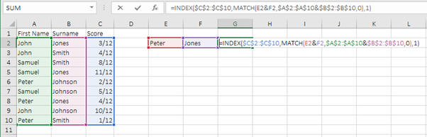
So in G2, we’ll create our formula.
Let’s start by indexing the range we want to return: C2:C10

=INDEX($C$2:$C$10,

To find the right row, we’ll need to match E2 (the first name) within A2:A10 and F2 (the surname) within B2:B10, so we’ll join the lookup values together (E2&F2) and the lookup arrays together (A2:A10&B2:B10). We’re only looking for an exact match, so we’ll use 0 (exact match) as the last argument for the match function.

=INDEX($C$2:$C$10,MATCH(E2&F2,$A$2:$A$10&$B$2:$B$10,0)

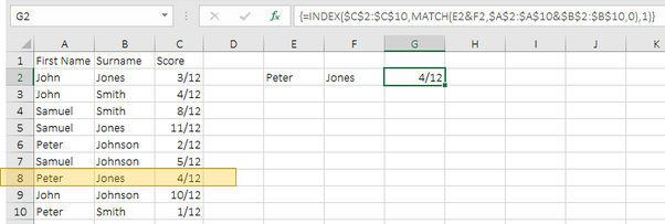
Once we’ve got the formula finding the right row, we’ll tell it which column to use (there was only one column in the indexed range, so we’ll have to use that):

=INDEX($C$2:$C$10,MATCH(E2&F2,$A$2:$A$10&$B$2:$B$10,0),1)

Once our formula is in, we’ll finish it off by turning it into an array formula by pressing CTRL+SHIFT+ENTER(so we get the curly brackets around the formula).

Note: don’t try to type the curly brackets, you need to use CTRL+SHIFT+ENTER.

If you want to refresh your knowledge on INDEX & MATCH first, you’re most welcome to have a look at my mini-course here before trying to master your first array.

Good Luck 🙂
As always; if you have a question on a specific Excel topic, you’re most welcome to send us an email.