DOC Office Consulting

Flash Fill is a feature that was new in Excel 2013 and it is absolute gold.

If you’ve ever had to extract just a small part of a cell throughout an entire list or had to join together parts of multiple cells within a large list, you’re going to absolutely love Excel’s flash Fill feature. It’s so simple, you’re going to save yourself bucket loads of time once you’ve mastered it (which’ll take all of about ten minutes – it really is that simple).

Here’s how it works…
Flash Fill will detect and replicate patterns in your data – so if there’s a logical pattern that you’re using to extract data, Excel can be told to use the same pattern.
For this example, I’ll use a list of names.

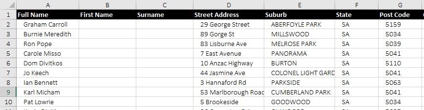
There’s actually 517 records in my list, but a small sample will work exactly the same as a large sample. The full name of each person is listed in column A, which is what will be used to seperate it into First Names in column B and Surnames in column C.
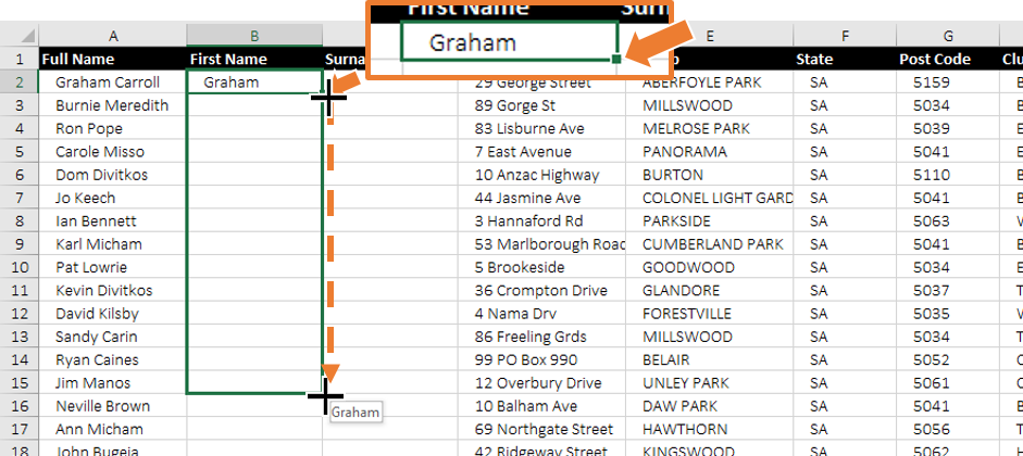
Instead of retyping 517 first names and 517 surnames, only the first first name needs to be entered (in B2). Once the first one is entered (checking that the spelling is accurate), select the cell that’s just been entered (B2), click the fill handle and drag down to fill down through the entire range (or double click the fill handle to automatically fill down).

By default, Excel will copy the first cell throughout the range, but a different fill option is easily chosen. Click the fill options box that pops up at the bottom of the filled range and select Flash Fill.

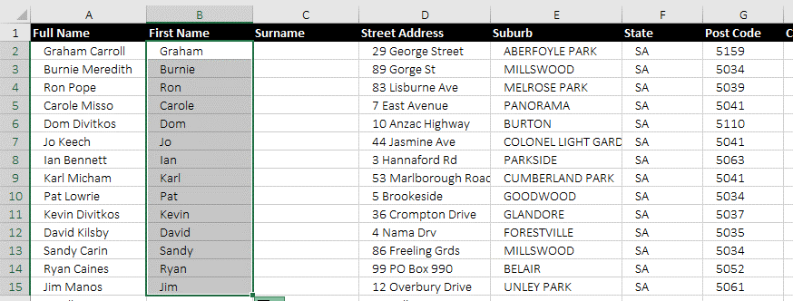
Excel detects the pattern in the data entered by comparing it to other cells in the same row and replicates it through the entire range (in this case the pattern is everything to the left of the space)– saving us having to retype 516 of the 517 names.

Repeat the process in column C to flash fill the surnames.

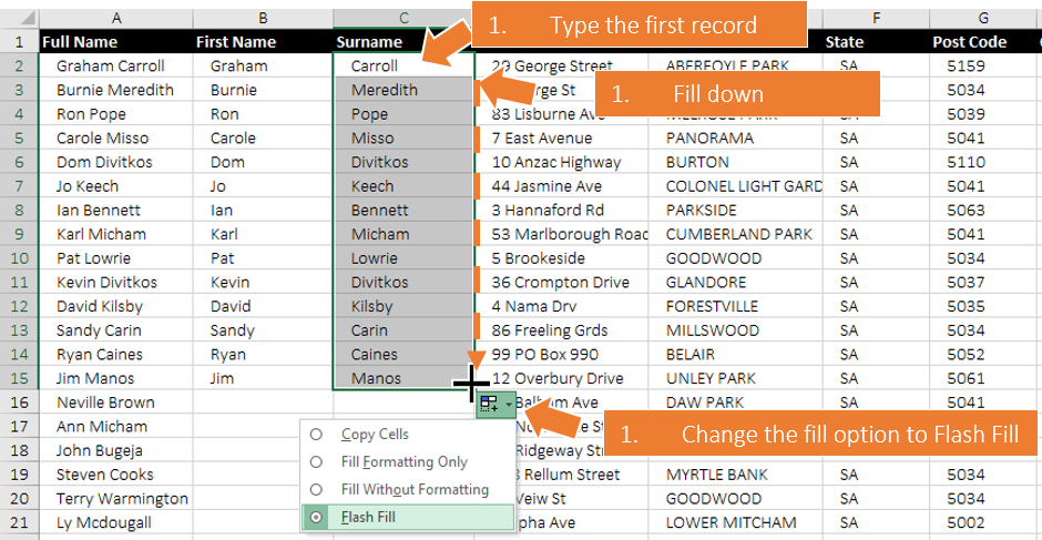
Again, Excel detects the pattern (everything to the right of the space) and replicates it throughout the range – saving us having to retype 516 of the 517 surnames.

See – I told you it was easy 🙂

If you’re a keyboard user…
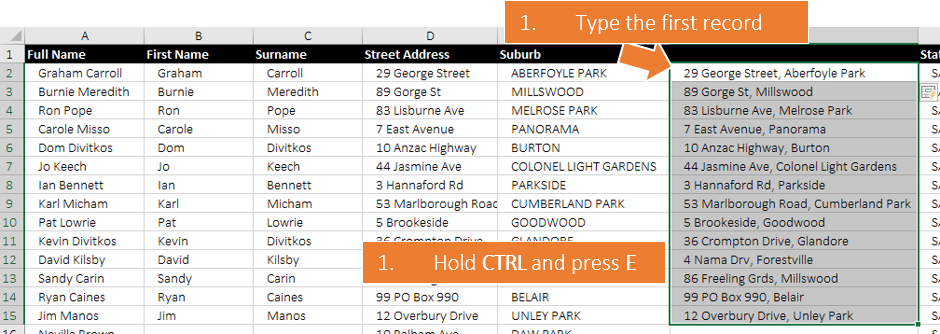
(for copying, pasting, filling, etc), rather than a mouse user, the keyboard shortcut CTRL+E will achieve the same result.

• Enter the first cell in the list
• With the cell just entered selected, Click CTRL+E

Note: to Enter without changing the selected cell, click CTRL+Enter after typing the first item, instead of just Enter

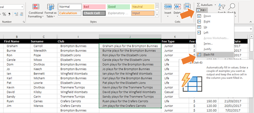
Or if you’re a ribbon user…

• Enter the first record
• Select the range from the first record through to the last record
• From the Home tab of the ribbon, select Fill, then choose Flash Fill

Personally, I prefer the keyboard shortcut because I am a typist, but you can choose whichever method you prefer – they all do the same thing.
As you might have noticed from the keyboard user example; flash fill can also be used to join cells together. The example concatenates the street address (from column D) and the Suburb (from column E).
And it can be used to concatenate cells with additional text that may not appear within the data (as shown in the example for Ribbon Users): (“Graham plays for the Brompton Bunnies”

As long as there’s a logical pattern that Excel can detect, it’ll replicate it. That pattern could be everything to the left of the space, everything to the right of the space, the first 4 characters of a cell, the year from a date cell, the 7th – 9th characters in a string, everything after a hyphen or comma… whatever you need. As long as there is a logical pattern for the extraction, Excel will replicate it.

How cool is that!
Go ahead, have a go and save yourself from wasting hours on unnecessary data entry.

If you’re using an older version of Excel (pre 2013), or you need the data to be extracted with a formula, you can check out my series of tutorial videos on text manipulation functions here – that walk you through achieving the same result with a formula.

Stay curious!
Dani xo