DOC Office Consulting

How can I create a dependent drop down list?
This is a question that I get all the time and while the question is simple enough – the answer is anything but. It’s going to require the creation of a dynamic named range that’ll use multiple functions nested within a single formula to make the range for our drop-down list truly dynamic. It’s also going to require your thinking cap – so go put it on.
Dependent Drop-down List within a Worksheet
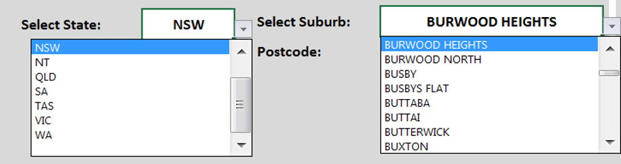
To keep it as simple as possible – I’ll use all the states of Australia in my first drop down list, and all of the suburbs within the selected state for my dependent drop-down list. Here’s my drop-down lists…
The second drop-down list will display different suburb options depending on the state selected in the first drop-down list.

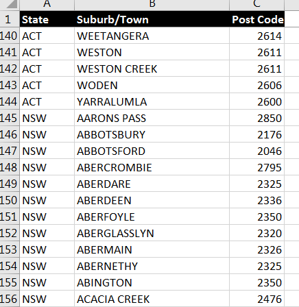
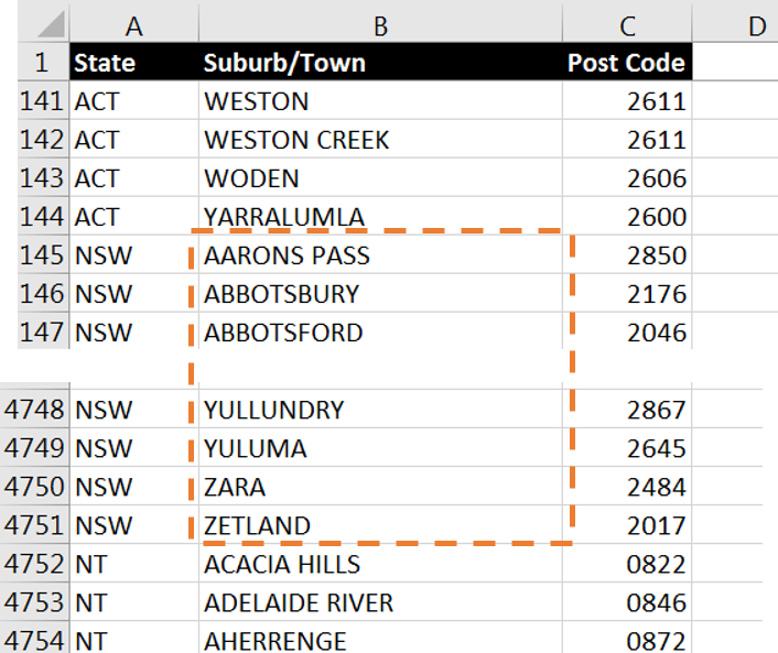
And here’s a snapshot of my source data (this is a very small snapshot, there’s actually 16,000 suburbs and towns listed, and it’s all sorted alphabetically by state and by suburb/town).

Let’s start by naming the whole list of State/Suburb/Postcodes – I have a pretty standard naming convention – a range of cells starts with rng and It’s followed by what it actually is – so I’ll call this rngSuburbs.
In order to create our next named range (the one that’ll use a formula to determine the range of cells it refers to), we’ll want to select an item from our first drop down list. I’ve selected NSW.
Now we get to create our named range…
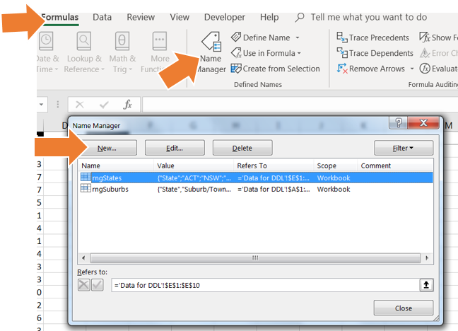
From the Formulas ribbon tab, click Name Manager. When the dialog box opens, select New

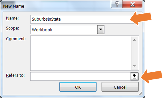
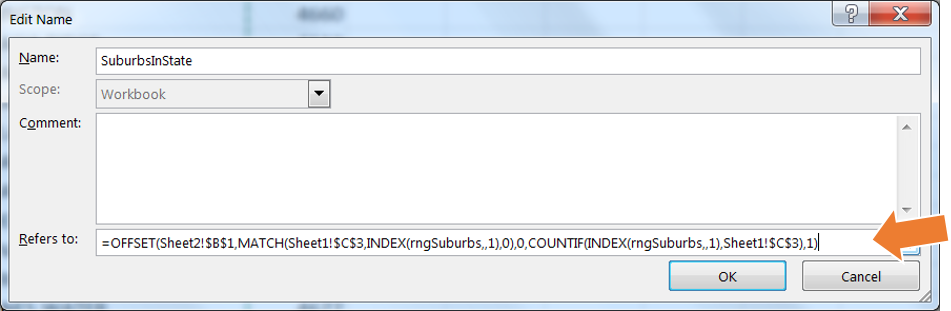
Here we’ll name our range (Note that I don’t prefix the name in this one with rng as it’s not a defined range of cells – it’s going to be a dynamic range of cells. I’ll call it SuburbsInState). And we’ll input the formula in the ‘Refers to’ field (you might want to click the pop out box to expand the area you have to type the formula)..

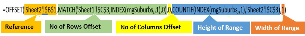
The formula that we’re going to create combines the functions OFFSET, MATCH, INDEX, COUNTIF and INDEX.

OFFSET

– How it works…
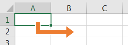
Using the Offset function, we can specify a single cell (the reference), then offset it by a certain number of rows and columns to actually refer to another cell. i.e. if we offset A1 by 1 row and 1 column – we would be referring to B2.

If instead of returning a single cell with OFFSET, we’d like to return a range of cells – we can input the height and width of the range. Let’s say the range should be 10 rows high and only 1 column wide. The formula that offsets A1 by 1 row and 1 column, that is 10 rows high and 1 column wide will now refer to the range B2:B11
Instead of referring to the range B2:B11 though, we want to refer to the range B145:B4751 (The first NSW suburb through to the last NSW suburb).
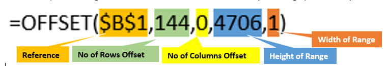
So our OFFSET function will need to OFFSET B1 by 144 rows and zero columns (to start at B145). It’ll need to be 4,706 rows high and 1 column wide. This will return the required range (B145:B4751).


That’s great…. If we know which row NSW starts on and we know exactly how many suburbs there are in NSW aand if we only want to return the suburbs of NSW… but we don’t. We want to use whichever state is selected – and of course each state starts on a different row and each state has a different number of suburbs – so we’re going to have to make our formula a bit more dynamic.

MATCH

– to Find the Starting Row
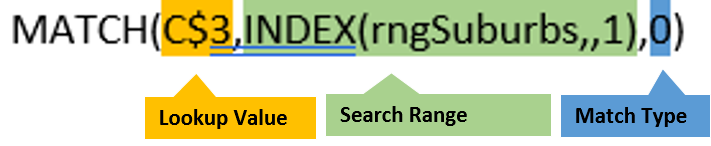
Instead of starting on row 145 every time, we need to know which row the selected state starts on and use this for the number of rows offset. To determine which row the selected state starts on, we’ll use a MATCH function. Match will return the position of the first cell with a matching value in a specified range – so we can look for the selected state, in the list of all states/suburbs/postcodes and find the position of the first cell.

Match needs 3 parameters:

1. What to look for (NSW)
2. Where to match it (the first column of the list of all states/suburbs/postcodes – conveniently named rngSuburbs)
3. Match Type – (0 for Exact Match)

This formula will return 145. Because the 145th cell of the range (rngSuburbs), displays the first matching entry. It’s going to work in exactly the same way if the user has selected SA instead of NSW; it’ll return the position of the first cell that matches SA in the range.

Fantastic!
So we can use this MATCH function as the Rows offset argument of our OFFSET function – to get the starting row of our range.

No of Columns Offset

The range that lists the suburbs in always in column B – so we don’t need to offset B1 by any columns. We’ll leave this argument with a zero value: 0.

COUNTIF

– to get the Height of Range
To determine the height of the range, we need to know how many suburbs are in NSW – or how many rows in the first column of the state/suburb/postcode list have the value of NSW. For this we can use a simple COUNTIF function.

The COUNTIF function will count all cells within a range that meet the criteria specified. It has just 2 arguments:

1. Range (range of cells to be checked for criteria)
2. Criteria

In our case, the range will be the first column of the state/suburb/postcode list (rngSuburbs) and the criteria will be the state selected in cell C3. This COUNTIF function will return the value 4,706 – the number of cells that have a value of NSW.

Brilliant!
So now we’ve created a dynamic function that we can use as the height argument of our OFFSET function.

Width of Range

The width of our range won’t change as all suburbs are listed in just 1 column, so we’ll simply use the value of 1 as the width argument.

Putting it all together

Let’s put our whole formula together. Start with the OFFSET function and use Sheet2$B1 as the reference, input the MATCH function into the Row Offset, 0 (zero) in the columns offset, the COUNTIF function in the Height, and 1 (one) in the width argument.

Now that we’ve created a formula that will return the correct range by returning the number of rows offset, the number of columns offset, the height of the range and the width of the range – and we know that these will recalculate nicely when another state is chosen – it’s time to put them all together and enter them into the ‘Refers To’ box in the name manager.

Creating the Drop-down List

Now that we’ve created our dynamic named range, it’s time to create the drop-down list that uses this named range as it’s source.
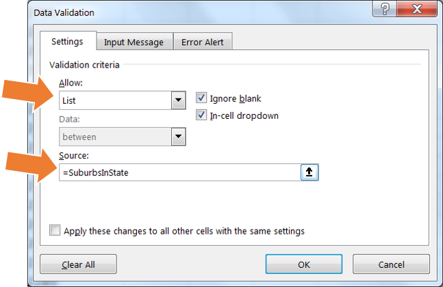
Select the cell where the drop-down list needs to go and from the Data tab on the ribbon, select Data Validation.
We’ll change what’s allowed to a List and we’ll specify the source of the list as the name of our dynamic range (SuburbsInState).

AWESOME!!
Now the second drop down list only offers items (suburbs) that belong to the category (state) that’s selected in the first drop-down list. Yay.
If you’ve made it through this one – and you have a vague understanding of what we’ve done – you’re doing better than most.
Alright, so I do know that this is all quite complex; which is why I’ve attached a workbook with the named range in it which you can download from this link. Feel free to download the file, test the dependent drop-down list and check out the functions of the named range. If you need a refresher or a more comprehensive instruction on the functions used – check out some of my free mini-courses here.
As always; if you have a question on a specific Excel topic, you’re most welcome to send us an email

Good Luck!
Dani xo