DOC Office Consulting

How can I colour code cells in Excel so that -10 is red and +10 is green?

With conditional formatting of course 🙂

Excel’s Conditional Formatting menu is choc full of tools to help you automatically format your cells based on their values or on the values of adjacent cells – or both! In this instance, I’d recommend using colour scales to create a heat-map.
With colour scales, you’ll specify 3 or 4 values and the selected cells will be shaded in a colour that’s determined by the value of the cells (the closer the cell value is to one of the specified values, the closer the cell colour will be to the specified colour).

How To Create a Heat-map

• Select the cells to be formatted
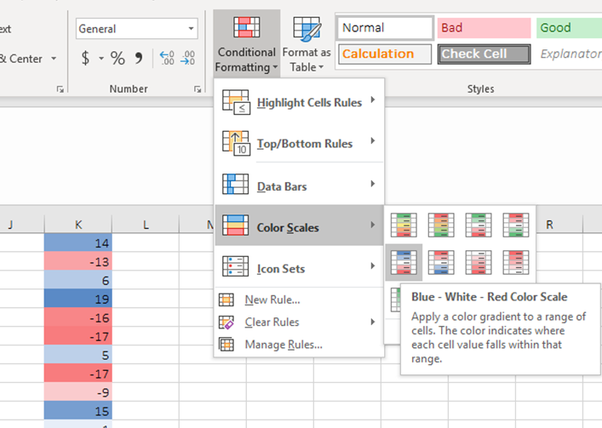
• Click the Conditional Formatting menu (on the Home tab of the ribbon)
• Select Color Scales and choose one of the options displayed (Blue – White – Red or whatever you prefer)

Blue – White – Red shows the highest result in blue, the mid point in white and the smallest in Red. You don’t have to be sold on the colour though – or the assumed values, we can easily change the properties once the rule has been created).

Once you’ve applied the color scales, Go back into the Conditional Formatting menu and choose Manage Rules.

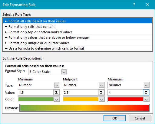
Here we can customise the colors and the values for which each color is applied. By default this style wants to colour the smallest value, the midpoint, and largest value with Red – White – Blue, but you can change it to a specific number (instead of smallest and largest) and a specific color (instead of the default) using the drop down lists.

• From the Conditional Formatting dialog box that opens, select the rule and click Edit Rules

• Under the heading minimum, change the Type from Lowest Value to Number, change the value to -10, and choose a colour from the colour drop-down selector
• Under the heading midpoint, change the Type from Percentile to Number, change the value to 0 (or whatever you prefer), and choose a colour from the colour drop-down selector
• Under the heading maximum, change the Type from Highest Value to Number, change the value to 10, and choose a colour from the drop-down selector

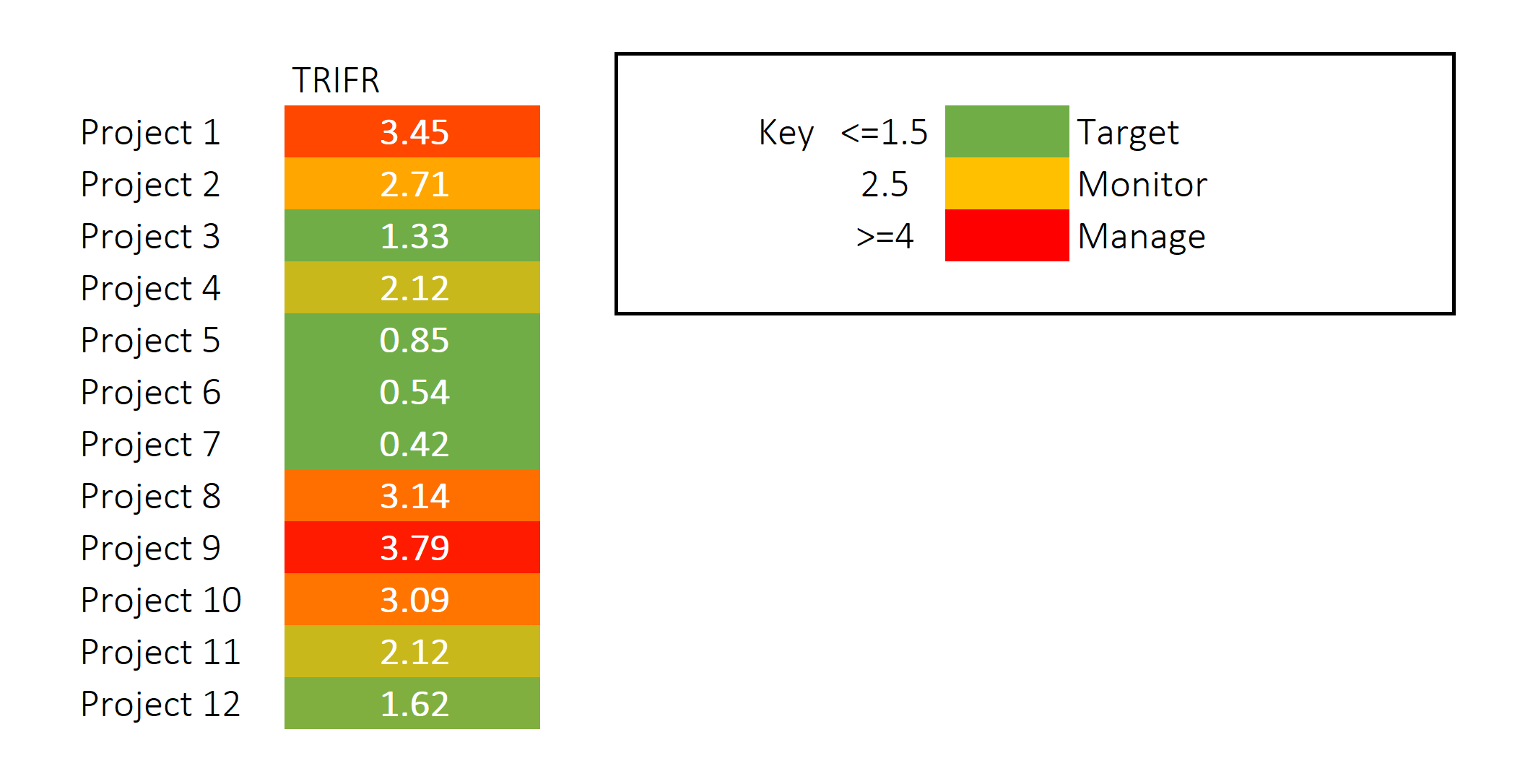
In my example, lower results are good and higher are bad, so I’ve used 1.5 as my minimum (with green for the colour), 2.5 as my midpoint (yellow) and 4 for my maximum (red)

• Click OK

Now it doesn’t matter how low the number gets, 1.5 and below will be formatted with the same colour chosen under minimum (green for me), 2.5 will be shaded with the same yellow, 4 and greater than 4 will be formatted with the exact same shade of the colour chosen (red for me) and all of the values in between will be graded – green through to yellow through to red, depending on how close to the specified values they are.

If you want to learn more about Excel’s Conditional Formatting tools – check out some of my free mini-courses here.
As always; if you have a question on a specific Excel topic, you’re most welcome to send us an email

Good Luck!
Dani xo