DOC Office Consulting

What formula could I use to extract only Unique items from a large table of data?
Great Question! There isn’t an Excel function that’ll do this for you (yet). You could to it with a pivot table, but sometimes that’s not practical, so if you really need a formula to return the results, you’re going to need an array formula
A word of caution – array formulas aren’t for the faint hearted; they’re quite tricky, but if you take the time to understand them, they’re well worth the trouble. All the little things you can’t do with a regular formula?… well they’re possible with an array formula.

Let’s have a look….
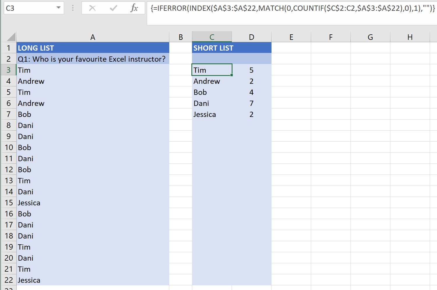
I have a list of survey responses in cells A3:A22 and it’s the same responses repeated again and again. I don’t really want to display a repeating list of the same items, I’d just like a short list of unique items and a summary showing how many times each response is recorded. This is how it’s going to appear once we’ve created our array formula:

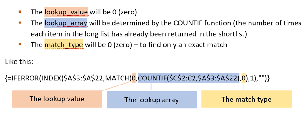
The array formula that we’ll use will combine INDEX, MATCH and COUNTIF all encased within an IFERROR function to return only unique items from a list. Here’s how it’s going to work:
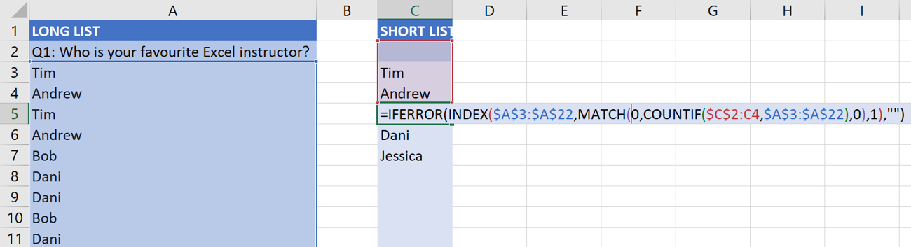
Entering this formula in C3, then filling down through the range C3:C22 will give us a unique list of items:
{=IFERROR(INDEX($A$3:$A$22,MATCH(0,COUNTIF($C$2:C2,$A$3:$A$22),0),1),””)}

And here’s how these functions will work:

• IFERROR will ensure that errors (#N/A when there are no unique items left) don’t display
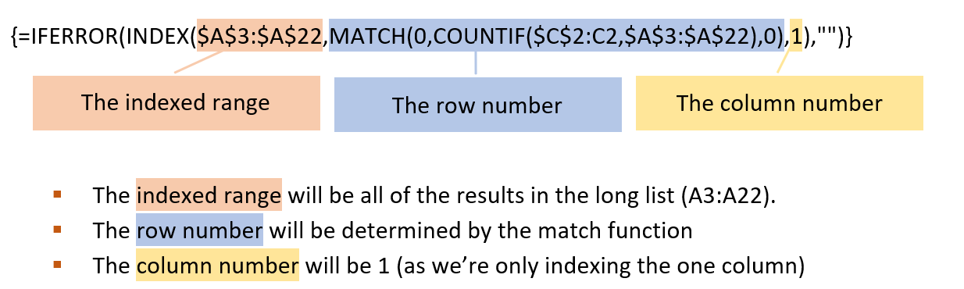
• INDEX will index the long list – as we want to return an item from this list
• MATCH will choose which row within the long list to return
• COUNTIF will determine how many times each item in the long list that has been added to the shortlist so far

Here’s how each of the functions work (and how they’ll work together in our array). If you’re already familiar with each of the functions, you can skip the Examples

IFERROR

The IFERROR function will evaluate the formula and if the formula results in an error, it’ll return the value_if_error instead of the error
{=IFERROR(INDEX($A$3:$A$22,MATCH(0,COUNTIF($C$2:C2,$A$3:$A$22),0),1),””)}

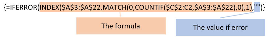
In this case, the value_if_error is blank (double inverted comma’s with nothing in between is a blank text string)

INDEX

Index will index a range of cells and return the value of the cell at the intersection point of a specified row and column within the range. So for our awesome formula, we just need to specify the Indexed range, the row number within the range and the column number within the range, like this:

Example of Index function:
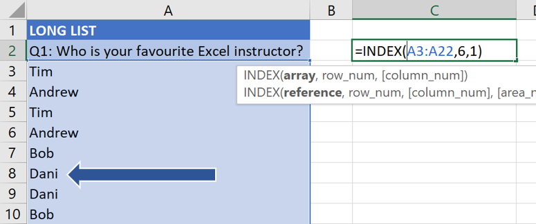
e.g. In the below image, the formula: =INDEX(A3:A22,6,1) has indexed the range A3:A22, and specified the cell to return as the intersection point of the 6th row and 1st column. **Note that it’s not the 6th row and 1st column within the worksheet, it’s the 6th row and 1st column within the indexed range (A8)

MATCH

Match will lookup a specified value in a range of cells (or an array) and return the position of the cell (or array item) that matches what it’s looking for. For our match function:

Example of Match function:
e.g. In the below image, the formula: =MATCH(“Dani”,A3:A22,0) will look for the value of “Dani” in the range of cells A3:A22, and return the position (within the range) of the cell with the matching value. **Note that it’s not the position within the worksheet, it’s the position within the range).

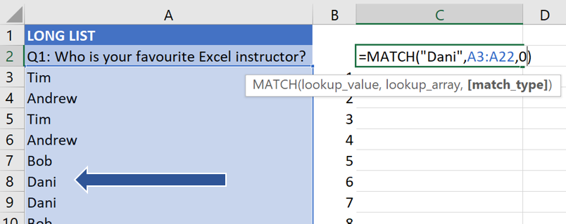
So this formula will return 6, as the values in the lookup range are: cell 1=”Tim” (no match), cell 2=”Andrew” (no match), cell 3 = “Tim” (no match), cell 4= “Andrew” (no match), Cell 5= “Bob” (no match), Cell 6 = “Dani” (match!), hence the MATCH function returns 6 as it finds the first match in the 6th cell within in the range. **Note that the cell within the worksheet that matches is A8, but our match function returns 6 – remember it’s the position within the range, not the worksheet – this is very important!

We’re going to come back to MATCH in a minute, once we’ve covered the COUNTIF (which is the lookup_array argument within the MATCH function)

COUNTIF

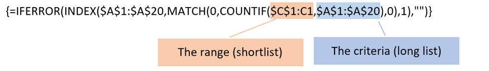
COUNTIF is going to determine the how many times each item in the long list has already been returned in the shortlist. Usually COUNTIF would only return one value (how many times a particular value appears in a range), but because we’re putting it in an array; it’s going to return multiple values (how many times each value appears in a range). Our COUNTIF is essentially going to perform multiple COUNTIF functions, with the range being the same each time and the criteria changing each time to each different cell in the criteria range.

• The range will be the shortlist (note that the shortlist is defined with a mixture of relative and absolute referencing – ensuring that it’s an increasing range that will grow by an additional row each time it’s copied down – more about that in a minute)
• The criteria will be determined by each cell in the criteria range

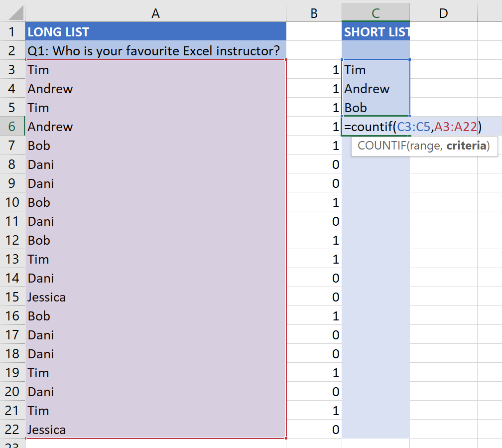
Example of Countif function:
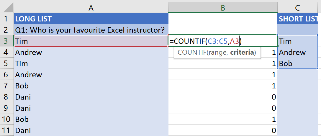
e.g. In the below image, the formula: =COUNTIF(C3:C5,A3) will count the number of times that the value of A3 (Tim) appears in the range of cells C3:C5, and return the number of cells that have a matching value (1).

By using a range of cells (all of the long list) for the criteria instead of a single cell, we can return multiple results in a single cell (the number of times each item in the long list appears in the short list).
e.g. In the below formula: =COUNTIF(C3:C5,A3:A22), our array will count the number of times that the value of each cell in the long list (the criteria range A3:A22) appears in the short list (range C3:C5), and return the result for each countif – the number of cells in the range that have a matching value to each criterion {“Tim”=1;”Andrew”=1;”Tim”=1;”Andrew”=1;”Bob”=1;”Dani”=0;”Dani”=0;”Bob”=1;”Dani”=0;”Bob”=1;”Tim”=1;”Dani”=0;”Jessica”=0;”Bob”=1;”Dani”=0;”Dani”=0;”Tim”=1;”Dani”=0;”Tim”=1;”Jessica”=0}), resulting in an array of values: {1;1;1;1;1;0;0;1;0;1;1;0;0;1;0;0;1;0;1;0}

By counting the number of times each item in the longlist appears in the shortlist, we can find the first item from the longlist that doesn’t appear in the shortlist, as the COUNTIF will result in 0 (zero) if it doesn’t already appear in the range.

Absolute and Relative Referencing

As the shortlist is being created by the formula, we can’t reference the entire shortlist within each formula – or all of the results will be the same (and include circular references), so we’re going to have to make the reference to the existing shortlist an increasing range (of all of the previous cells in the list) by cleverly creating a mixture of relative and absolute references.

• In the cell C3 (the first formula), our shortlist should only include in the cell C2 ($C$2:C2)
• In C4, (the second formula) our shortlist should include all of the cells in the shortlist above C4: C2:C3 ($C$2:C3)
• In C5 (the third formula), our shortlist should again include all of the cells in the shortlist above C5: C2:C4($C$2:C4)

Are you seeing the pattern here?
The range always starts in C2, but the last cell in the range needs to grow to encompass one more row each time. The way we create an increasing range like this is to make the beginning of the range absolute (with dollar signs to lock it in), like this: $C$2, but make the last cell in the range completely relative (without dollar signs), like this C2. So when we create our shortlist range (in C3) we will reference the range of cells $C$2:C2 – even though our initial range only spans one cell, we still need to make it a range so that when this formula is copied down, the first cell will stay the same (because it’s absolute), but the range will increase by one row each time (as the end of the range is a relative reference).

PUTTING IT ALL TOGETHER

With our long list in the range A3:A22, we’ll enter the first formula in C3 and fill it down, but I’m going to illustrate how the formula works in cell C5 (so we already have a couple of values in our short list)…

COUNTIF: we’ll use the result of the COUNTIF (array) function to determine how many times each item in the long list appears int the short list
In cell C5: This is the COUNTIF portion of the formula: COUNTIF($C$2:C4,$A$3:$A$22)Which evaluates to:{1;1;1;1;0;0;0;0;0;0;1;0;0;0;0;0;1;0;1;0}(by performing multiple COUNTIF functions (one for each item in the criteria range (the long list))

MATCH: The Match function will find the first item in the COUNTIF array that has a zero value:
This is the MATCH portion of the formula: MATCH(0,COUNTIF($C$2:C4,$A$3:$A$22),0). After evaluating the COUNTIF function, this is what the MATCH function is evaluating: =MATCH(0,{1;1;1;1;0;0;0;0;0;0;1;0;0;0;0;0;1;0;1;0},0), which will evaluate to: 5 (as it finds the first zero in the 5th item in the array)

INDEX: The Index function will return the value of the cell in the position determined by the MATCH function.
In C5, this is the INDEX portion of the formula: INDEX($A$3:$A$22,MATCH(0,COUNTIF($C$2:C4,$A$3:$A$22),0),1).
After evaluating the COUNTIF function, the INDEX function is evaluating this: INDEX($A$3:$A$22,=MATCH(0,{1;1;1;1;0;0;0;0;0;0;1;0;0;0;0;0;1;0;1;0},0),1).
After evaluating the MATCH function, the INDEX function is simply evaluating this: INDEX($A$3:$A$22,5,1) and evaluates to “Bob”

IFERROR: While C5 isn’t going to result in an error, when we get further down the list (to cell C8), there aren’t going to be any items in the COUNTIF array that have a zero value, hence the MATCH function will return an error, so encasing it all in IFERROR ensures those nasty #N/A results won’t be displayed.
Once you’ve finished inputting your formula, make sure you complete it by pressing CTRL+SHIFT+ENTER, so that Excel puts in the curly brackets. **Note that typing the curly brackets won’t work – you need to press CTRL+SHIFT+ENTER.

SUMMARY OF RESULTS

COUNTIF
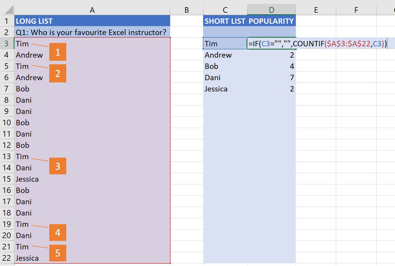
To create a short summary showing how many times each item appears in the long list, we’ll simply create a basic COUNTIF formula in cell D3.
In the below image, the formula: =COUNTIF(A3:A22,C3) will count the number of times that the value of C3 (Tim) appears in the range of cells A3:A22, and return the number of cells that have a matching value (5).
IF
I’ve encased my COUNTIF within an IF function to ensure that it’s only performing the count in rows where a unique item has been returned, and returning a blank cell in the count column, if there’s a blank cell in the same row in the shortlist.

And that’s how you create a list of unique items with a formula !

That was hard work wasn’t it? I did warn you that array formulas aren’t for everyone.
I’ve attached a workbook with the example I’ve used that you can download here and work through to help you get your head around it, but in order to make a formula like this work – you really do need to understand INDEX & MATCH. If you’d like a refresher on those functions, you can sign up for my mini-course here – it’s free, and you also need to apply what you’ve learnt to your own data – taking the time to understand how each of the functions work.

Go on… if you’ve made it this far – you should have a go. Yes, it’s tricky but you’ll be rewarded for your efforts when your future data manipulation takes you a tiny fraction of the time that it takes everyone else 🙂

Cheers,
Dani xo